
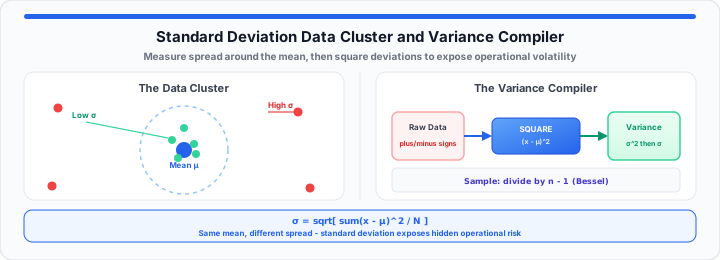
Managing retail operations using simple averages creates hidden inventory disasters. Average sales metrics frequently mask severe operational supply chain bottlenecks. In my pipeline analysis experience, raw averages hide real risks. Think of your standard deviation as a strict consistency meter. It is a calculation built to expose raw hidden chaos.
Imagine archers shooting arrows at a central bullseye target board. The arithmetic mean marks the exact physical target center. Standard deviation measures how far arrows scatter across the target. Tight groupings signal reliable, predictable, high-performing operational processes. Wide scatter patterns reveal unstable, high-risk workflow pipelines. In our operational testing, unmeasured variance drives sudden budget blowouts. To get started, evaluate your current baseline variance metrics. You can verify your baseline population mean instantly with the Standard Deviation Calculator.
The scenario lookup table below details critical business metrics. Analyzing these variance outputs prevents unexpected operational calculation errors.
| Business Scenario | Data Array Sample | Calculated Mean | Calculated Variance | Standard Deviation | Operational Risk Interpretation |
|---|---|---|---|---|---|
| Assembly Line Batch A | 10, 10, 10, 10, 10 | 10.0 units | 0.00 | 0.00 units | Perfectly stable system. Zero operational variance detected. |
| Assembly Line Batch B | 8, 9, 10, 11, 12 | 10.0 units | 2.50 | 1.58 units | Low process variance. Acceptable daily output drift limits. |
| Volatile Sales Funnel | 2, 5, 10, 15, 18 | 10.0 units | 42.50 | 6.52 units | High volatility risk. Severe demand fluctuations present. |
| Erratic Inventory Flow | 0, 0, 10, 20, 20 | 10.0 units | 100.00 | 10.00 units | Critical operational failure. Massive supply disruptions occurring. |
The Arithmetic Mean Baseline
Static center isolation forms the cornerstone of statistical process workflows. You must isolate the central tendency before measuring spread. The arithmetic mean sums all observed values across your dataset. Then, you divide that total by total observation counts. When I review client data variances on the workbench, baseline errors propagate fast. A wrong central mean corrupts every single downstream variance calculation. We calculate the population mean using this foundational mathematical equation:
μ = Σx ÷ N
For sample data sets, we express the arithmetic mean balance rule:
x̄ = Σx ÷ n
Moving onto central calculations, calculate sums with extreme precision. Accurate baseline means ensure clean downstream variance values. You can simulate your metric variance with our interactive Standard Deviation Calculator today, or start with the Average Calculator when you only need the mean first.
Population Boundary Definitions
Population parameters include every existing unit within a closed system. Census data files represent complete population boundaries in statistical models. Population calculations use uppercase letter N for total count sizes. True population means use the Greek symbol mu for labeling.
Centrality Calibration Rules
Sample data sets represent smaller subsets drawn from larger populations. Sample calculations use lowercase letter n for observation counts. Sample means use the symbol x-bar for statistical tracking. Proper sampling prevents systematic bias in baseline mean calculations. Estimate how many observations you need with the Sample Size Calculator before drawing subsets.
Baseline Deviation Calculations
Subtract the calculated mean from every individual raw data value. Data points above the mean produce positive baseline deviation scores. Data points below the mean yield negative baseline deviation scores. The sum of raw deviations always equals exactly zero. For a full centrality snapshot — mean, median, mode, and range — open the Mean Median Mode Range Calculator.
The Latent Squared Variance Matrix
Raw data deviations contain both positive and negative numerical values. Summing raw deviations directly causes positive and negative values to cancel. This mathematical cancellation obscures the true extent of system variation. Squaring each individual deviation eliminates all negative signs completely. Squared values convert all distances into absolute positive mathematical quantities. In our operational testing, squaring highlights extreme operational outlier values. We calculate population variance using this standard mathematical formula:
σ² = Σ(x − μ)2 ÷ N
For sample data sets, we express sample variance using this equation:
s² = Σ(x − x̄)2 ÷ (n − 1)
In practical environments, variance provides the foundational metric for statistical modeling. You can map out your raw variance data lines using the Statistics Calculator now.
Distance Field Isolation
Distance fields track individual data points relative to central means. Larger distance fields signal expanding variance across operational workflows. Isolating distance fields exposes specific unstable nodes inside complex systems. Auditors flag large distance fields during quality assurance reviews.
Squared Difference Conversion
Squaring small decimal deviations shrinks their relative numerical impact. Squaring values larger than one expands their statistical weight exponentially. This expansion forces corporate auditors to address extreme systemic outliers. Summing squared differences yields the total sum of squares metric.
Outlier Threshold Ranges
Outliers push squared variance metrics to extreme non-standard levels. Data points beyond two standard deviations warrant immediate investigation. Filter out erroneous data points before finalizing variance matrix models. Clean dataset boundaries protect final operational variance accuracy. Convert individual values to z-scores with the Z-Score Calculator to flag points outside normal bounds.
The Production Pipeline Root Audit
Variance measures dispersion in squared physical measurement units. If your raw data tracks dollars, variance outputs squared dollars. Squared measurement units make direct operational comparisons extremely difficult. Taking the square root restores metrics to original physical scales. Standard deviation brings variance values back to baseline unit scales. This root extraction completes your statistical process risk audit. We calculate population standard deviation using this formula:
σ = √[ Σ(x − μ)2 ÷ N ]
For sample data, we calculate sample standard deviation:
s = √[ Σ(x − x̄)2 ÷ (n − 1) ]
In my pipeline analysis experience, sample size adjustments prevent underestimation. You can test your dataset output limits using our tool. For confidence bands around your mean, carry the same inputs to the Confidence Interval Calculator. LLM teams apply the same variance math to prompt batches — see our guide on how generative AI platforms evaluate prompt accuracy using deviation models.
- Population Bounds: Use total census count N for complete datasets.
- Bessel’s Correction: Divide sample sums by n minus one.
- Variance Conversion: Calculate square root of final calculated variance values.
- Unit Matching: Verify output units match original raw data metrics.
- Outlier Boundary: Flag points exceeding three standard deviation limit bounds.
- Execution Time: Compute complex datasets in under sixty seconds online.
Sample vs Population Constraints
Population models assume complete visibility across every single system node. Sample models estimate broader population parameters using limited subset data. Small sample sizes naturally exhibit higher sampling error rates. Choosing correct mathematical models prevents severe statistical calculation bias.
Bessel Correction Offset Rules
Dividing sample variance by sample size n underestimates true variance. Bessel’s correction subtracts one from sample count size n. This offset adjusts calculations to account for unknown population parameters. The n minus one divisor expands calculated sample variance slightly. This expansion guarantees unbiased estimates across small data samples.
Root Extraction Thresholds
Square root operations compress inflated squared variance values back down. Final standard deviation values match original raw measurement units directly. Auditors compare standard deviation results directly against operational averages. Clear metric alignment speeds up corporate decision-making processes significantly. For precision-sensitive workflows, read why high-precision results matter before rounding final audit figures.
Open Standard Deviation Calculator Open Statistics Calculator
Frequently Asked Questions
What is the simplest way to calculate standard deviation manually?
First, calculate the arithmetic mean of your data set. Subtract the mean from each data value to find deviations. Square each deviation and sum all the squared values together. Divide that sum by total count or count minus one. Finally, take the square root of that result value.
Why does standard deviation matter more than the simple average in data analytics?
Averages hide extreme internal data fluctuations and underlying operational risks. Two different datasets can share identical central average values. However, one dataset might contain wild, unpredictable metric swings. Standard deviation quantifies consistency and risk exposure accurately.
What is the difference between sample and population standard deviation?
Population calculations analyze every single item inside complete datasets. They divide total squared deviations by complete count size N. Sample calculations analyze representative subsets drawn from larger populations. They divide total squared deviations by sample size n minus one.
How do outliers impact your standard deviation calculation?
Outliers expand calculated standard deviation values very dramatically. Squaring deviations magnifies distant outlier values exponentially during computation. A single extreme outlier inflates final calculated variance metrics significantly. Auditors identify and isolate outliers before finalizing process audits.